Tuesday, July 2, 2024

Determining the shortest Site-to-Shoreline path. Considerations.

 “A common mistake is to assume, implicitly or explicitly, that Bronze Age and modern coastal morphology are essentially the same.” [1]


Well (pace Tartaron) we have to start somewhere. 

In order to understand the possible relationship of Bronze Age sites both to the sea and to nodes of trade a good first step would be to determine the straight line distance between each BA site and the nearest seacoast.  By examining a map on which such straight-line links are plotted we can begin to understand the relationship of such sites to the shoreline and the focusing effect that shoreline irregularities have in mapping inland sites to the sea.  First, however, we must have a model of the seashore of sufficient accuracy to allow us to say with some confidence what those distances are and we have no choice but to start with the modern shoreline.  A picture should make these initial themes clear.

Figure 1. Straight lines drawn from BA sites in Arcadia to the nearest seashore.


In this map I have projected (straight-line) each BA site in Arcadia onto the nearest seacoast.   Arcadia is entirely landlocked and its communication with the greater outside world is through neighboring territories; Messenia and the Gulf of Messenia to the S near modern Kalamata, across Triphylia to the W and the Gulf of Kyparissia, and across Achaea to the N (perhaps near ancient Helike).  The primary contact between Arcadia and the ocean is through the southern Argolid near the head of the Gulf of Argos.  It is this concentration of land-to-sea contacts created by the closest gulfs and inlets that I am speaking of.  An accurate representation of site-shoreline direct lines will make this concentration effect clear and it will fulfill another function: that of classification.  We would like an easy way of generating lists of onshore sites as distinct from those inland

But how is this to be done with a database and software?  The first thing that is required is an accurate representation of the shoreline for the entire Bronze Age world.

In the end I decided to make my own.   To be sufficiently accurate the nodes should be no more than 20 m apart for the area being mapped.  The region of Locris is a good example of the technique that I adopted.  Here is an image of the coast of Locris:

Figure 2.  The shore of Locris (Euboea at the top).

First let us superimpose on this map a representation of the database BA sites in this area:

Figure 3.  The north coast of Locris with BA sites as white squares.

Here the sites are represented by white squares.  The problem now is to create a straight line from each site to the nearest seashore irrespective of any land obstacles, mountains, canyons, rivers, etc.  The algorithm adopted should be sufficiently rigorous to be reasonably convincing.  To draw a line to a point withing 30 m of the ‘ideal and perfect’ location should be rigorous enough.  In most cases we can do better than that.  But how should  this be done?

The algorithm I chose was as follows:

a.    Trace by hand the outline of the several land masses

b.   Each node in this line had to be 30 m or less from the next node.

c.    Produce software that would try each (and every) site against all the outline nodes until it found the smallest distance. 

d.   The output of this software would be a set of sql insert statements for a new table, coast, that would hold, for each site, the minimum distance to the shore along with the lat/lon coordinates for the location on the shore closest to the site.

e.    Modifying the production software to generate a distance to shoreline report from the  coast table.  I described this report in my last blog post.

What did this process look like.  In Google Earth Professional I generated a ‘path’ structure that would follow the coast.  When visible, I followed the wet sand mark along the coast.  It looked like this:


Figure 4. Kamares Beach on Sifnos. 
The red dots are interpolated coastal points.


In this figure we see the Paralia Kamares on Sifnos (36.990171° N, 24.678167° E).  I have interpolated a coastline for this beach (blue line).  My interpolated points are the red dots.  The beach is 525 m long (I used the yellow segmented line to measure it) and the dots divide the beach into 67 segments.  Each node (dot) therefore is separated from the next by ~7.83 m.  The next figure shows a detailed view:

Figure 5.  Detail of Kamares Beach.


In figure 4 the yellow measuring line has been removed and the reader will get a better idea of the spaces between the nodes (red dots on the blue coast line).

The site closest to Kamares Beach is C7406, which is a Sanctuary of the Nymphs on Sifnos.  The minimum distance from this sanctuary to the closest shoreline is ~508.8 m.  Given tides, erosion, and other factors the figure should be accurate to +/- 5 m (503.8 to 513.8 m) at worst.


Figure 6. Detail of closest marker to C7406.


In this extreme closeup we see the specific node that marks the closest approach of the shoreline to C7406.  Its next nearest node on the left is  ~15 m.  From C7406 to the closest node is an angle of 332.56°.  To the next closest point on the left the azimuth is 330.81°.  So, an angular displacement of something over 1.75° per node and a lateral error distance of about 15 m. arises from this scheme.   Other sites will provide widely varying parameters of distance and angle but I present this example of C7406 as a typical case and it is this sort of accuracy or better which I have striven for in all the coast tracing exercises I have undertaken.

Which Approach?

I began this extended coastal exercise with the assumption that the entire coastline of the several land masses and islands had to be traced in detail.  In Crete I attempted to trace the entire coastline.  The yellow outline in the next picture represents what I was able to accomplish:

Figure 7.   Crete.  The yellow outline represents my attempt to trace the coast.

Even this (not entirely satisfactory) outline required 8000 points placed by hand.  It required several days of steady work but, in the end, I decided that this approach has serious drawbacks.  First of all the human factor of such eye-straining repetitive work is a drawback.  Second, even 8000 points do not result in the accuracy which I desired to achieve.  The coastline of Crete is about 985 km (985000 m).  Dividing this figure by 8000 gives an average distance between nodes of about 123.1 m.  This is about six times worse than the accuracy given for the Sifnos example above.   There 
would need to be at least 48000 nodes in the outline of Crete in order to render both a complete outline of Crete and one which was of sufficient accuracy to use for closest shoreline point determination.  I was forced to abandon one criterion or the other and I decided to jettison the idea of creating complete outlines of the landmasses the eastern Mediterranean and just concentrating of those stretches of coastline most likely to be closest to BA sites.

To create an accurate least-distance placing (and with minimal effort) it is necessary to center a circle on each site and note where that circle touches the coast.  Then we draw detailed coastline nodes only at these specific points.  This approach immediately dispenses with having to outline projecting capes and peninsulas since these are highly unlikely to be the closest points to anything.  Here is an example.

Figure 8. Eupalion (C562) in Phocis. Corinthian Gulf

In figure 8 the site of Eupalion/Gouva (C562) is represented by the square rectangle in the center.  Centered on that rectangle is a red circle that just touches the shoreline.  The coastal outline (blue line) is only elaborated in the vicinity of the red circle.  Now it is only necessary to place one or more nodes around the tangent of circle/line segment.  This results in considerable time savings and accuracy is enhances.  In the neighborhood of the intersection of the red circle and the coast it might pay to lay  down points that are much closer together and so ensure greater accuracy.


.  Figure 9.  Southern Phocis on the Gulf of Corinth

In figure 9 C562 (Eupalion) is on the left and two more sites in southern Phocis (C563, C564) are on the right (east).  The coast outline only touches the coast at spots where the closest shoreline has already been determined by circles centered on the sites themselves.  Proceeding in this way means that most the rugged south coast of Phocis will not require modeling in this typical example.

In the example of Crete that I mentioned achieving the desired accuracy with the ‘whole coast model’ approach requires about 48000 points in the shore outline.   As there are 1500+ sites on Crete the computational cost will be 48000 * 1500 or 72,000,000 separate distance computation routine calls.  If we allow only 10 points per site using the previously described circle-focus method then it would require only 15000 outline points and so 1500 * 15000 = 22,500,000 routine calls – a computational savings of about 2/3.   This would run is something under 2 minutes on GoDaddy's servers which is where I run this utility-type software.

Another approach is to take advantage of the fact that Crete is divided into subregions in the Mycenaean Atlas database and so it's possible to model just one region at a time.  This would considerably reduce and spread out the workload into manageable chunks.

Figure 10.  Gulf of Atalantis.  Northern Locris.


Figure 10 is an example of the circle-focus method as I applied it to Northern Locris.  Here the sites are represented by white squares.  Each is the center of a circle which extends to the closest coastline.  The blue line is the coast outline.  Notice that it only touches the shoreline where the circles do.  Only those segments are carefully modelled.  The rest of the line is ‘armature’.  The software algorithm adopted for calculating the minimal distance traverses this entire blue outline (node to node) and, for each site, returns that distance along with the lat/lon  pair of that specific closest point on the coast.  In figure 11 we see what that this same region of Locris looks like after processing and with the shortest distance lines properly placed.

Figure 11. North coast of Locris with lines
drawn from sites to nearest seashore.

I represent the nearest approach of site to seashore with a blue line that starts at the site (indicated by a diamond) and ends at the closest seashore point (indicated by a red circle).

These are some of the considerations that I had in mind when performing the task of automating the task of finding the closest seashore to every BA site.  The reader should keep in mind that the ‘shortest distance’ is not from the site, exactly.  It measures the distance from my site marker to the seashore.

In another blog post I would like to discuss what algorithm my software used and whether there are any other useful coastal outline databases available.


Footnotes

[1] Tartaron [2017] 140.


Bibliography

Tartaron [2017] : Tartaron, Thomas F.,  Maritime Networks in the Mycenaean World.  Cambridge University Press,  ISBN: 978-1-108-43136-1.  Paperback edition of 2017.


Sunday, June 23, 2024

On the Beach

 I am happy to announce that the users of the Mycenaean Atlas now have the ability to examine distances from Bronze Age sites to the closest shoreline.

The main control page now features a new way for the user to specify a low and high distance. 

The new control is in the lower center.


Here is the new control in close-up:


 Having specified the range the user will see a new page that displays distances in four ways: a map of the returned sites, a list of the sites with distances to the shore, a histogram in which the sites are distributed into 'same distance' buckets, and a line chart in which the sites are lined up in distance order.


Analysis of sites within 1000 m of the shore.


For example you may be interested in all sites within 1000 m of the shore.  You specify 0 as the minimum distance, 1000 as the maximum distance and then you click on submit.  The resulting four-part display will show you all sites within 1000 m of the closest shoreline: on a map, in a list, in a histogram, and on a line chart.

It may not be optimal to display the entire DB in this way; more researchers are interested in examining one island or region at a time.  The control allows for that.  If you want only to examine the Cyclades then you will type 'Cyclades' into the text input labelled 'Region' (and specify a range).  


When you click submit you will see that the display is limited just to the Cyclades.  

Result of selecting just the 'Cyclades'.


This atlas considers individual islands as 'subregions'.  If you wished to look just at Naxos in the Cyclades then type 'Cyclades' for the region and 'Naxos' for the subregion.


Selecting 'Cyclades' and 'Naxos' from the control


The analysis page for Naxos.


The individual place key site detail page has also been modified.  Now if a distance to the ahore is defined for the site then there will be a label on that page that says 'Distance to Shore (click)'.  When you click on that label a map will pop up that shows the site with a line drawn to the nearest shoreline.  Click on the map to pop it back down.


Click on this to see site to shore map.


The site to shore map with connecting line.  Zoomable.
Click on map to pop it down
.


The concept of shoreline poses some problems.  'Shoreline' is a dynamic concept and no precision is ever possible.  There are the tides, of course.  Distance to nearest shoreline depends on the time of day.  And while I give figures precise to the decimeter the real distance may fluctuate tens of meters depending on the time of day.  Here in the United States we have a joke about the State of Rhode Island which is said to be '5% larger at low tide.' There have also been dramatic changes in the shoreline since the Bronze Age.  There is the case of Tiryns, of course.  Formerly on the water's edge it is now more than a kilometer inland.  Rivers have done their usual work in the last 3500 years.  What were formerly islands are now landlocked by deltas as is the case for Aetolia-Acharnania.  And there have been changes even more dramatic.  The city of Helike in Achaea was drowned by earthquake and land subsidence in 373 BC.  There have been changes in the ocean level which, combined with land subsidence, have led to differential variations in shorelines across the E. Aegean world.  Nisakoula in Messenia is an illustrative case.  Once a thriving settlement it is now submerged.  Likewise Paulopetri in Laconia.  The filling in of the Cothon harbor near Nestor's Palace in Messenia has placed that Palace further from the ocean than it would have been in the tthieteenth century BC.  So the accuracy of my figures can certainly be questioned and in very few cases are they even accurate to within 10 m.

  So if I cannot achieve absolute accuracy with my distances why, then, have I provided them?  My readers should consider the 'distance to shoreline' as a classifying device.  This new ability will quickly allow users to create lists of sites 'on the shore' (0 to 1000 m, say), 'a moderate distance from the shore' (2 to 5 km?), and 'inland sites' (perhaps sites further from the shore than 6 or 7 km).  It would be very difficult to generate these classes in any other way.  Why should my users care about these classes?  Well, for one thing, distance from the coast might very well be reflected in diet and occupation.  And there are obvious effects on the type of work that communities might perform.

How was this done and how were these figures arrived at?  The first step in such work is to create a new DB table just to store site identifiers and distances.  Populating such a table is the next step.  This consisted of drawing in Google Earth an outline of all the areas involved.  Such an outline consists of nodes and vertices.   This is time-consuming and I experimented with different approaches.  For Crete I traced the entire shoreline - some 4000+ nodes.  For areas such as Attica I used a circle and node technique.  In this method I drew circles centered on the various sites and only modeled those stretches of coast where the circles touched the shoreline.  This resulted in significant savings in both time and labor

I then wrote a .php routine that would calculate the distances from each site to ALL the nodes and save the shortest distance along with the corresponding lat/lon pair for that point/node on the shoreline.  In this system, as implemented, there is one and only one 'closest point' for each site even though many sites have access to the shoreline at two or more points at nearly identical distances.  Some of these access points that are a little further away are objectively better for ocean access than the closest point.  I save these difficulties for later discussion.  In a potential refinement the current table could be combined with the data from Arthur de Graauw's harbor data.

This work of outline tracing is not yet completed.  The areas that are done are

  • Achaea
  • Arcadia
  • Argolid
  • Attica
  • Boeotia
  • Corinthia
  • Elis
  • Laconia
  • Macedonia
  • Megaris
  • Messenia
  • Thessaly

Among the islands the work is completed for

  • Antiparos
  • Crete
  • Euboea
  • Kasos
  • Kephalonia
  • Kos
  • Lesbos
  • Melos
  • Naxos
  • Paros
  • Rhodes
  • Syros
  • Thasos
  • Thera


    Monday, March 4, 2024

    Segment Ro of the Cyclopean Wall is located again


      The segment of the Cyclopean wall which was named 'Ro' by Broneer (Mycenaean Atlas Project: C7760) has been relocated by my colleague, Peter Barkevics. Its coordinates are 37.913475° N, 23.003006° E. It sits at an elevation of 27 m and is about 125 m. in a straight line on a bearing, from St, of ~273.1°. It sits on an open hillside about 20 m. above a large private home with a gray ('blue' in the photo) roof. Here is a picture of the situation.


    Hillside with Ro.  North at the top. Red line is the Hexamilion wall.
    Google Earth Image.


    Next is Barkevics' photograph of Ro looking directly east and downhill towards the house with the gray roof (which appears to be blue under open sky light) (37.913466° N, 23.003295° E).

    Section Ro of the Cyclopean wall. 
    Facing E and downhill.
    Peter Barkevics.  All rights reserved.


    In this picture the view is directly E; the house with the blue roof is clearly seen. On the left hand side can be seen the four projecting stones of Broneer's 'tower'. The other flanking stones are to the right. Compare this photograph to Broneer's drawing:


    Drawing from Broneer [1966] 350, Fig. 2, no. 4.


    In the next photo we see these stones from the other direction (looking west):


    Section Ro of the Cyclopean wall. 
    Facing W and uphill.
    Peter Barkevics.  All rights reserved.


    In this photograph the four projecting stones are now on the right. The large anchor stone visible in Broneer's drawing is at the lower left.


     That anchor stone is also clear in this next photo which looks at the east end of this segment while facing south.  Here the two east-side projecting stones (the 'tower') are on the right and stretching out towards the viewer.


    East end of section Ro of the Cyclopean Wall. 
    Viewer facing S.
    Peter Barkevics.  All rights reserved.


    Bibliography

    Broneer [1966] :  Broneer, Oscar. ‘The Cyclopean Wall on the Isthmus of Corinth and Its Bearing on Late Bronze Age Chronology’, Hesperia: The Journal of the American School of Classical Studies at Athens (35:4). 1966.  Online here.

    Broneer [1968] : Broneer, Oscar. 'The Cyclopean Wall on the Isthmus of Corinth, Addendum', Hesperia: The Journal of the American School of Classical Studies at Athens (37:1), 25-35.  The American School of Classical Studies at Athens. 1968.

    Gregory [1993] : Gregory, Timothy E., Isthmia V. The Hexamilion and the Fortress, American School of Classical Studies at Athens. Princeton, New Jersey. 1993. ISBN: 0-87661-935-9.

    Kardara [1971] : Kardara, Chrisoula. 'The Isthmian Wall; (A Retaining Wall for a Road)', Athens Annals of Archaeology (4:1), 85-89. 1971.  Online here.

    Morgan [1999] :  Morgan, Catherine. Isthmia VIII; The Late Bronze Age Settlement and Early Iron Age Sanctuary. The American School of Classical Studies at Athens, Princeton, New Jersey. 1999.

    Simpson and Hagel [2006]:  Simpson, R. Hope and D.K. Hagel. Mycenaean Fortifications, Highways, Dams and Canals. SIMA vol. 133. Paul Ã…ströms Förlag. Sävedalen, Sweden. 2006.


    Sunday, February 18, 2024

    Photographs of section Pe of the Cyclopean Wall

     I mentioned in a previous post that my associate, Mr. Peter Barkevics, has confirmed the location of segment Pe of the 'Cyclopean' wall near Isthmia in Greece.  The position of this segment is 37.913457° N, 22.997472° E.

    Fig. 1.  Area of the Isthmus.  Blue way-mark
    indicates section Pe of the 'Cyclopean' wall.

    Zooming in:

    Fig. 2.  Area of the 'Cyclopean' wall.  Section Pe is in the center
    at the blue way-mark.

    Section Pe was reported by Oscar Broneer in 1966 [1] and he provided a drawing of it:[2]

    Fig. 3.  Broneer's drawing of section Pe of the 'Cyclopean' wall.


    Overlaying the site re-established by Barkevics with Broneer's drawing gives this:

    Fig. 3a.  Google Earth image overlaid with Broneer's sketch of Pe.  Broneer [1966] 350, fig. 2, no. 3.  Elevation of the wall at the way-mark is 60 m. a.s.l.

    This wall segment is about 6 m from the edge of the modern road.

    Broneer described Pe like this: 

    "One continuous stretch, Pe (Fig. 2,3; Pl. 81), in the property of Sotiris Peras, measures 45.50 m. in length. Only the outer, northern face is well preserved, in places to a height of two courses, but a few stones from the inner face show that the wall here had a thickness of 3.60-4.00 m. The stones are large, some measuring 1.50-1.75 m. in length and 0.75 m. in height.  There are four towers, varying in width between 2.10 and 2.60 and projecting ca. 0.70 m. from the face of the wall. The distance from one tower to the next varies between 7.90 and 9.50 m.  There was very little earth close to the wall, and the sherds found on the surface are mostly small pieces of undatable coarse fabrics. Two undecorated pieces might be Mycenaean."[3]

    Two previous photographs of Pe are known to me - one appeared in Broneer [1966] [4].  The other appeared in Morgan [1999]. [5]  To these old and now outdated photographs Mr. Barkevics has added some fifty color photos which detail the segment stone by stone.  At the bottom of this next figure we see Mr. Barkevics diagram notes of the positions where his pictures were taken and, above that, my own diagram that tries to match his photos to Broneer's drawing.


    Fig. 4.  Upper drawing is Broneer [1966] 350, Fig. 2, no. 3.
    Lower drawing is Google Earth overlaid with Barkevics' way markers.

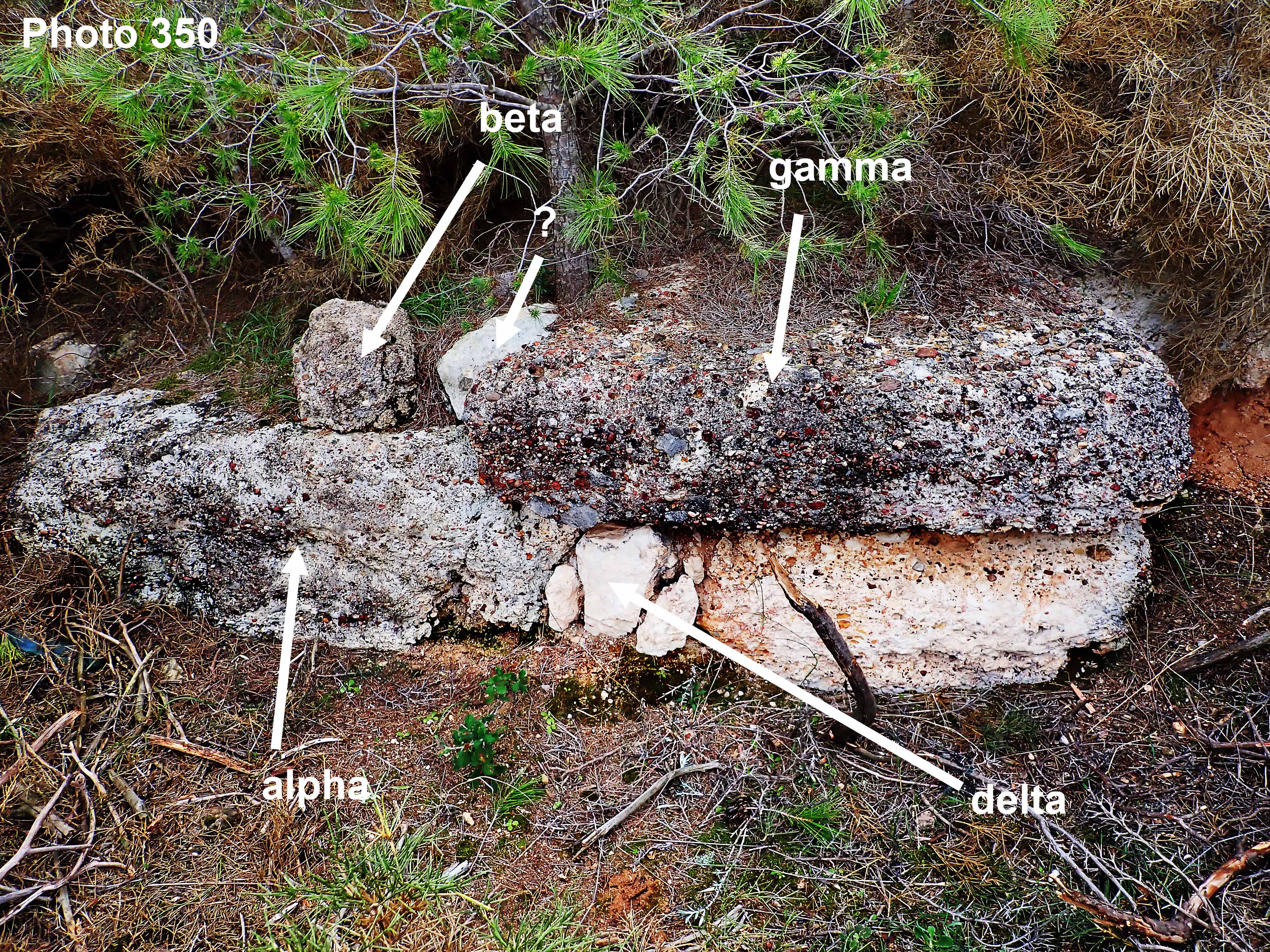
    Is this segment photographed by Barkevics the same as that shown in Broneer's photo?  Yes.  This next photo shows my labels for several of the stones in the Broneer photo:

    Fig. 5.  Broneer [1966] Pl. 81.


    This next photo by Barkevics shows the same stones with corresponding labels:

    Fig. 6.  Tower 3 (from W).  View is to S.


    I believe that stone beta has been moved and I may not have identified it correctly.  Stone beta may actually be the next small stone (with the question mark) to the viewer's right.  The other stones are clearly the same.

    Following is a tour of the structure from the west to the east.

    Fig. 7.  Photo 325.  The first two stones of the N face on the west. 
    Viewer is looking S.

    This photo shows the first two stones in the sequence, starting from the west.  This is photo 325 and you can see its position by looking at the left side of fig. 4 in this post.  Here are the same two stones again (note the mossy patch).


    Fig. 8.  Photo 326.  West end of N face.  View facing S. 
    The person is standing on the north edge of the modern road.

    Fig. 9.  Photo 327.  First tower from the W.

    This is the first (counting from the W) of the projections which Broneer identified as 'towers'.  Their small size and the nature of the ground strongly suggest that they are buttresses.  

    The next photo shows the view from the N of this same 'tower'.

    Fig. 10.  Photo 328.  Same tower from the N and looking S.


    The second 'tower' from the left is shown in the next photo:

    Fig. 11.  Photo 332.  Tower 2 (counting from the W).


    ... and another view of Tower 2:

    Fig. 12.  Photo 333.  Tower 2 from a bit further back.

    The next photo gives another view of Tower 3 (already shown in Fig. 6):

    Fig. 13.  Photo 346.  Tower 3.  The view is to SE. 
    Ten-euro note (127 x 67 mm) for scale.

    Another view of Tower 3:

    Fig. 14. Photo 348.  Tower 3 from N. 
    View is directly S.  Compare to Fig. 5.


    Fig. 15.  Photo 351.  East end of Tower 3 (from W).


    Fig. 16. Photo 357.  Tower 4 (counting from the W).  View from the E.
    Underbrush suppressed for clarity.

    It is difficult to escape the impression that section Pe is slowly being degraded by natural forces.  Both erosion and the undergrowth (particularly pine trees) are going to dislodge more stones.  The Archaeological Service might do a great deal of good by spending a day clearing brush around this very important monument.

    In future blog posts I will publish more of Barkevics photos and then try to say what we have learned about the Cyclopean wall.


    Footnotes


    [1] Broneer [1966] 351.

    [2] Broneer [1966] 350, fig. 2, no. 3.

    [3] Broneer [1966] 351

    [4] Broneer [1966] Plate 81.

    [5] Morgan [1999] 443, fig. 8.  Mislabelled 'Section Sp'.  The correction is due to Simpson and Hagel [2006] 130, fn. 103.


    Bibliography

    Broneer [1966] :  Broneer, Oscar. ‘The Cyclopean Wall on the Isthmus of Corinth and Its Bearing on Late Bronze Age Chronology’, Hesperia: The Journal of the American School of Classical Studies at Athens (35:4). 1966.  Online here.

    Broneer [1968] : Broneer, Oscar. 'The Cyclopean Wall on the Isthmus of Corinth, Addendum', Hesperia: The Journal of the American School of Classical Studies at Athens (37:1), 25-35.  The American School of Classical Studies at Athens. 1968.

    Kardara [1971] : Kardara, Chrisoula. 'The Isthmian Wall; (A Retaining Wall for a Road)', Athens Annals of Archaeology (4:1), 85-89. 1971.  Online here.

    Morgan [1999] :  Morgan, Catherine. Isthmia VIII; The Late Bronze Age Settlement and Early Iron Age Sanctuary. The American School of Classical Studies at Athens, Princeton, New Jersey. 1999.

    Simpson and Hagel [2006]:  Simpson, R. Hope and D.K. Hagel. Mycenaean Fortifications, Highways, Dams and Canals. SIMA vol. 133. Paul Ã…ströms Förlag. Sävedalen, Sweden. 2006.


    Friday, February 16, 2024

    Section St of the 'Cyclopean' Wall is found

     Peter Barkevics, has re-established the location of segment St of the 'Cyclopean Wall'. [1]  It is at 37.913404° N, 23.004431° W.  Formerly this was on an olive grove owned by the Statiris family.[2]  After being described by Broneer et al, some years ago, it was acquired by its present owners.  The wall is positioned in the front yard of a bed and breakfast.  Some stones appear to be occluded by building in the back of the property.  This section of the wall is 237 meters from segment Sk on a bearing, from Sk, of 282.79°.

    The owner allowed Pete to photograph freely but would only allow two reduced-size images to be reproduced on this blog.

    North face of St looking W


    North face of St looking E


    All photographs are the property of Peter Barkevics and all rights are reserved.

    In this next photo we see the B&B property as it looks in Google Earth:


    Here is a copy of the drawing that Broneer made of St.[3]

    In this final photo I superimpose Broneer's drawing over a GoogleEarth image of the B&B in question.


    Here I have fit the drawing to the stones as best I could. It seems clear that the north face runs E-W through the center of the lawn. The south face is partly covered by the driveway and, in the back, by the building of a shed.

    Peter Barkevics has interesting observations about the current condition of this wall. He writes:

    "The current owner, ..., says there have been several floods of water from Mytika area after heavy rain in past years. A culvert has been built between the houses above his and it discharges over his courtyard. The discharge has eroded some of the area and the wall was affected. ... All I can say is that a quick survey of the site by the archaeological service would be a good idea. It's only a day's work for a survey team ... "

    I want to thank Peter for his untiring work in finding and documenting these wall fragments.  They are important for understanding Greece's Late Helladic history. Shamefully they have so far been given, not analytical, but mythologizing treatment.

    Footnotes

    [1] First described by Broneer and Kardara. For section St see Morgan [1999] 440, no. 2, 'Section St (Statiris Property)'. Also Broneer [1966] 349 and fn. 8.

    [2] Broneer [1966] 349.

    [3] Broneer [1966] 350, fig. 2, no. 5.

    Bibliography

    Broneer [1966] :  Broneer, Oscar. ‘The Cyclopean Wall on the Isthmus of Corinth and Its Bearing on Late Bronze Age Chronology’, Hesperia: The Journal of the American School of Classical Studies at Athens (35:4). 1966. Online here.

    Kardara [1971] : Kardara, Chrisoula. 'The Isthmian Wall; (A Retaining Wall for a Road)', Athens Annals of Archaeology (4:1), 85-89. 1971.  Online here.

    Morgan [1999] :  Morgan, Catherine. Isthmia VIII; The Late Bronze Age Settlement and Early Iron Age Sanctuary . The American School of Classical Studies at Athens, Princeton, New Jersey. 1999.


    Blog Posts Concerning the Isthmian Wall

    Since 2023 a number of posts concerning the Isthmian Wall and how we located its remaining segments, have appeared on this blog.  This post ...